Quotation Format in Excel: Free Template with GST Formulas

Download quotation-format.xlsx (free, no sign-up). The workbook has four sheets.

• How to use. Short instructions. Delete this sheet before you share the file. It is the only place our name appears.
• GST quotation. The main document, with HSN or SAC codes and the tax split.
• Simple quotation. The same layout without GST, for unregistered businesses.
• Items. Your item list: description, HSN or SAC, unit, rate and GST %. It comes with three sample rows so the document sheet shows live numbers when you first open it.

Yellow cells are for typing. Everything else in the item table is a formula. The file opens the same way in Microsoft Excel, Google Sheets and LibreOffice Calc, because it uses only basic functions and no macros.

The layout mirrors a printed quotation from top to bottom, so what you see on screen is what prints.

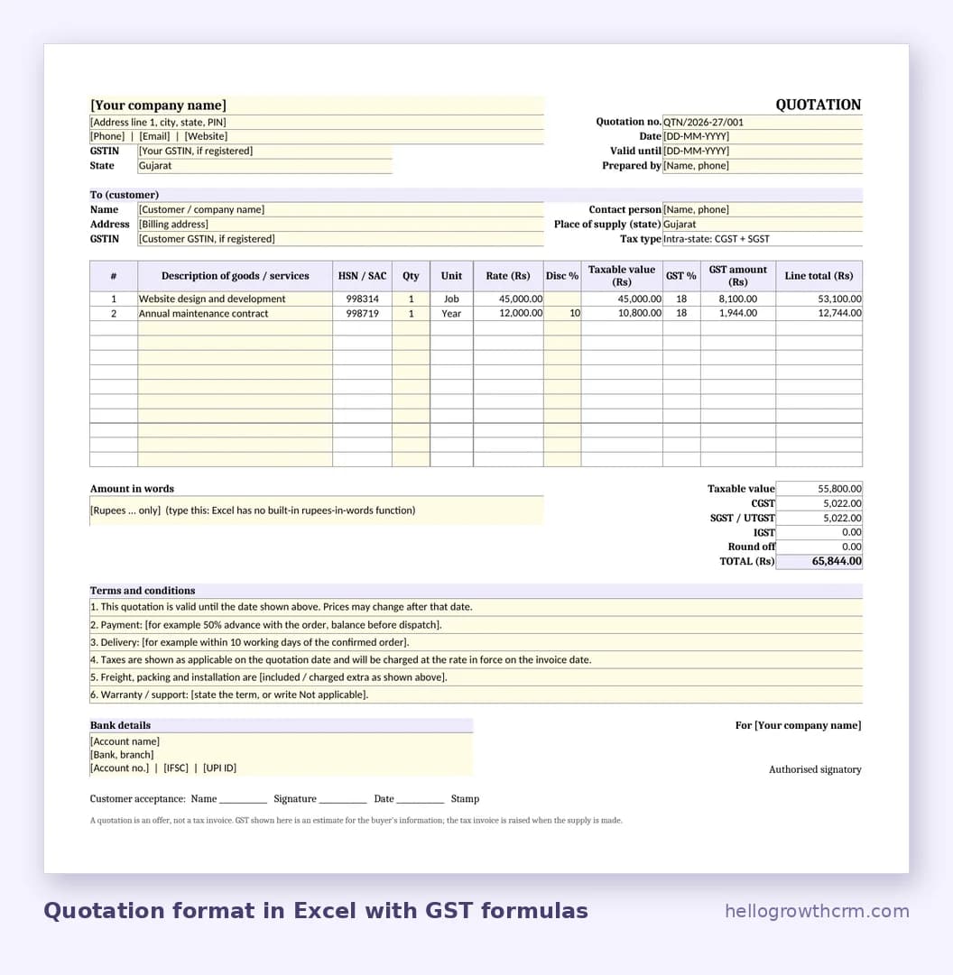
Row 13 is the first item row. Rows 14 to 24 carry the same formulas with the row number changed. Each formula starts by checking for an empty row, which is why unused rows stay blank instead of showing zeros or errors.

Three choices in those formulas are worth understanding before you change anything.

The discount sits inside the taxable value

H13 multiplies quantity by rate and then by one minus the discount percentage. GST in J13 is then worked out on that reduced figure. This is the treatment that carries through to the tax invoice, where a discount shown on the document reduces the taxable value.

ROUND is used on every money cell

Without ROUND, Excel keeps fractions of a paisa that you cannot see, and the column total can differ from the visible figures by a paisa. Rounding each line to two decimals makes the printed numbers add up exactly.

IFERROR keeps typed descriptions working

If you type a description that is not on the Items sheet, VLOOKUP finds nothing and IFERROR returns a blank instead of an error. Type the rate and GST % over the formulas in that row and the rest of the line still calculates.

The tax type is never typed. It is decided by comparing two cells: your state in B5 and the place of supply in I9. UPPER and TRIM make the comparison ignore capital letters and stray spaces, so gujarat and Gujarat match.

Spell the state the same way in both cells. If you would rather remove the chance of a spelling mismatch, replace both with two-digit GST state codes, such as 24 and 27, and the formulas work unchanged.

The file opens with two sample lines so you can confirm the formulas before trusting them with a real quotation. Your state and the place of supply are both set to Gujarat, and both items carry 18% in the Items sheet.

The sheet should show a taxable value of ₹55,800.00, CGST of ₹5,022.00, SGST of ₹5,022.00, IGST of zero, no round off and a total of ₹65,844.00. Now change the place of supply to Maharashtra. CGST and SGST drop to zero, IGST becomes ₹10,044.00, and the total stays at ₹65,844.00. If your copy shows anything else, a formula has been overwritten.

1. Open the Items sheet and replace the three sample rows with your own items, HSN or SAC codes, units, rates and GST rates. There is room for fifty.
2. On the GST quotation sheet, type your business name, address, contact line, GSTIN and state into the yellow cells at the top.
3. Edit the six lines of terms to match how you actually trade: advance, delivery time, freight, warranty.
4. Save this prepared copy as your master. In Excel, File, Save As, Excel Template (.xltx) makes every new quotation open as an untitled copy, so the master is never overwritten.
5. For each quotation, open the template, fill in the customer block and the items, and save it under the quotation number, for example QTN-2026-27-014.xlsx.

The most common way a quotation template goes wrong is a typed number landing on top of a formula. Protection prevents it. Select the yellow input cells, open Format Cells, Protection, and untick Locked. Then choose Review, Protect Sheet, and confirm. Now only the input cells accept typing. In Google Sheets the equivalent is Data, Protect sheets and ranges, with the input ranges listed as exceptions. Leave the password blank unless you need one, because a forgotten password locks you out of your own template.

The document sheets are already set to A4 portrait and fit to one page. In Excel use File, Print, and choose Microsoft Print to PDF, or File, Save As, PDF. In Google Sheets use File, Download, PDF. Send the PDF to the customer and keep the workbook yourself. If you want the yellow shading gone before printing, select the sheet and set Fill Colour to No Fill. The formulas are not affected.

Excel has no worksheet function that writes a number as rupees in words. The familiar workaround is a VBA macro, which forces the file to be saved as .xlsm. Macro files are blocked by many mail servers and do not run on phones, where a large share of quotations are opened. A typed cell is less clever and always works. If you want it filled in automatically, the online quotation maker writes the amount in words for you.

A workbook is the right tool while one person sends a few quotations a week. It starts to cost orders when three things happen at once: more than one person is quoting, customers ask for revisions, and nobody can say which quotations are still open. Excel has no idea a quotation was sent, so it cannot remind anyone to call.

At that point the quotation belongs in the same place as the customer record and the follow-up. In HelloGrowthCRM the quote builder uses your item list the way the Items sheet does, and quote tracking shows every open quotation with its value and next follow-up date. Our comparison of CRM vs Excel is honest about when the spreadsheet is still the better choice. Paid plans start at ₹899 per user per month, and there is a free plan: see India pricing.

The same workbook layout is available for two other documents: proforma invoice format in Excel and estimate format in Excel. For the layouts themselves, see the seven quotation formats, the proforma invoice format, the estimate bill format and the quotation letter format. Once the quotation is out, the guide to following up B2B quotations covers what to do next.